Observation input#
Observation input consists of a number of different inputs:
Observation files with correct name and content
Command Line Options
Preprocessor Variables
Observation files#
Observation files for TSMP-PDAF are netCDF files which follow a
certain naming convention. Each observation file has a fixed prefix
followed by the formatted number of the assimilation cycle which is
determined by da_interval . Additionally,
the command line input delt_obs determines the number of
assimilation cycles/iterations/steps that are run purely forward
before checking an observation file again.
The prefix is chosen with the command line option
obs_filename.
Example: If the chosen prefix is myobs, the observation files are
named myobs.00001, myobs.00002, myobs.00003, etc.
General observation file variables#
All observation files contain the following variable:
dim_obs#
dim_obs: (int) The observation files contain one dimension named
dim_obs which should be set equal to the number of observations for
the respective assimilation cycle.
dampfac_state#
dampfac_state: (real) Input of a time dependent state damping
factor. The damping factor for an update is given in the corresponding
observation file. This damping factor applies only to updates of
dynamic states in the DA-state vector and, when existing, replaces the
general input from
PF:dampingfactor_state.
dampfac_param#
dampfac_param: (real) Input of a time dependent state damping
factor. The state vector for an update is given in the corresponding
observation file. This damping factor applies only to parameter
updates in the DA state vector and, when existing, replaces the
general input from
PF:dampingfactor_param.
ParFlow observation file variables#
If TSMP-PDAF is only applied with ParFlow, the following variable
arrays of dimension dim_obs have to be specified in the observation
files:
obs_pf#
obs_pf: (real, dim=(dim_obs)) Observations for ParFlow (either pressure or soil
moisture)
obserr_pf#
obserr_pf: (real, dim=(dim_obs)) Observation errors which can be
different for individual observations (optional). If this variable is
not present. the command line option rms_obs (see Command line
options) will be used to define the observation error (equal for
all observations).
ix#
ix: (integer, dim=(dim_obs)) Position of the observation in the ParFlow grid in
x-direction.
iy#
iy: (integer, dim=(dim_obs)) Position of the observation in the ParFlow grid in
y-direction.
iz#
iz: (integer, dim=(dim_obs)) Position of the observation in the ParFlow grid in
z-direction.
idx#
idx: (integer, dim=(dim_obs)) Index of the observation in the ParFlow grid.
The positions are always relative to the south-east corner cell at the
lowest model layer. The index idx can be calculated as follows:
\begin{gather*} idx = (iz-1) \cdot nx \cdot ny + (iy-1) \cdot nx + ix \end{gather*}
where nx and ny are the number of grid cells in x- and y-direction
respectively and ix, iy and iz are the positions of the
observation in x-, y- and z-direction.
gw_indicator#
gw_indicator: (integer) Indicates if the observation is a pressure
observation. Values: 0, 1.
0: Soil water content observation (i.e. no pressure)1: Pressure observation
Used only for gwmasking=2 (mixed state vector). When pressure
observations are present, the state vector variable at the observation
location and below is set to pressure (it may have been set to soil
water content before).
ix_interp_d#
ix_interp_d: (real) Offset of the correct observation locations
compared to the position of the observation in the ParFlow grid
assigned with ix. Only used when
DA:obs_interp_switch is set to 1.
The correct observation location should be located at
\begin{gather*} x_{obs} = x_{grid}(ix) + \mathtt{ix_interp_d} \cdot \Delta x \end{gather*}
where
Important:
0 <= ix_interp_d < 1.\(x_{obs}\): x-coordinate of the observation location
\(x_{grid}(ix)\): x-coordinate of grid cell with index
ixin the ParFlow grid. Note that \(x_{grid}(ix) = \max_{ix}\{x(ix) | x(ix) < x_{obs}\}\) (closest grid point that is smaller than \(x_{obs}\))\(\Delta x\): Difference of x-coordinate between grid cells neighboring observation location: \(\Delta x = x_{grid}(ix+1) - x_{grid}(ix)\)
Example#
This example shows how to set ix_interp_d from a given (1) grid and
(2) observation location.
Let the observation location be at longitude \(x_{obs} = 6.404\).
Let the grid be simple going from 6.3 to 6.5 in steps of 0.02.
Example grid locations:
\(x_{grid}(1) = 6.3\)
\(x_{grid}(6) = 6.4\)
\(x_{grid}(11) = 6.5\)
We find ix and ix_interp_d as follows:
Find the two grid locations with longitudes closest to the observation location: \(x_{grid}(6) = 6.4\), \(x_{grid}(7) = 6.42\)
Choose the index of the grid location smaller than \(x_{obs}\) for observation file input
ix:ix=6Compute
ix_interp_dfrom the two closest grid locations as follows
\begin{gather*} \mathtt{ix_interp_d} = \frac{ x_{obs} - x_{grid}(ix)}{ \Delta x} \end{gather*}
Here this leads to ix_interp_d=0.2.
We can check this by computing \(x_{obs}\) from ix, ix_interp_d:
\begin{align*} x_{obs} &= x_{grid}(6) + \mathtt{ix_interp_d} \cdot \Delta x \ &= 6.4 + 0.2 \cdot 0.02 = 6.4 + 0.004 = 6.404 \end{align*}
iy_interp_d#
iy_interp_d: (real) Offset of the correct observation locations
compared to the position of the observation in the ParFlow grid
assigned with iy. Only used when
DA:obs_interp_switch is set to 1.
The correct observation location should be located at
\begin{gather*} y_{obs} = y_{grid}(iy) + \mathtt{iy_interp_d} \cdot \Delta y \end{gather*}
where
Important:
0 <= iy_interp_d < 1.\(y_{obs}\): y-coordinate of the observation location
\(y_{grid}(iy)\): y-coordinate of grid cell with index
iyin the ParFlow grid. Note that \(y_{grid}(iy) = \max_{iy}\{y(iy) | y(iy) < y_{obs}\}\) (closest grid point that is smaller than \(y_{obs}\))\(\Delta y\): Difference of y-coordinate grid cells neighboring observation location: \(\Delta y = y_{grid}(iy+1) - y_{grid}(iy)\)
Example#
This example shows how to set iy_interp_d from a given (1) grid and
(2) observation location.
Let the observation location be at longitude \(y_{obs} = 50.910\).
Let the grid be simple going from 50.8 to 51.0 in steps of 0.02.
Example grid locations:
\(y_{grid}(1) = 50.8\)
\(y_{grid}(6) = 50.9\)
\(y_{grid}(11) = 51.0\)
We find iy and iy_interp_d as follows:
Find the two grid locations with longitudes closest to the observation location: \(y_{grid}(6) = 50.9\), \(y_{grid}(7) = 50.92\)
Choose the index of the grid location smaller than \(y_{obs}\) for observation file input
iy:iy=6Compute
iy_interp_dfrom the two closest grid locations as follows
\begin{gather*} \mathtt{iy_interp_d} = \frac{ y_{obs} - y_{grid}(iy)}{ \Delta y } \end{gather*}
Here this leads to iy_interp_d=0.5.
We can check this by computing \(y_{obs}\) from iy, iy_interp_d:
\begin{align*} y_{obs} &= y_{grid}(6) + \mathtt{iy_interp_d} \cdot \Delta y \ &= 50.9 + 0.5 \cdot 0.02 = 50.9 + 0.01 = 50.910 \end{align*}
CLM observation file variables#
If TSMP-PDAF is only applied with CLM, different variable arrays of
dimension dim_obs (exception dr of dimension 2) have to be
specified in the observation files:
obs_clm#
obs_clm: (real, dim=(dim_obs)) Observations for CLM.
Default: Soil moisture observations.
obserr_clm#
obserr_clm: (real, dim=(dim_obs)) Observation errors which can be
different for individual observations (optional). If this variable is
not present. the command line option rms_obs (see Command line
options) will be used to define the observation error (equal for
all observations).
lon#
lon: (real, dim=(dim_obs)) Longitude of the observation.
lat#
lat: (real, dim=(dim_obs)) Latitude of the observation.
layer#
layer: (integer, dim=(dim_obs)) Index of CLM depth layer where the observation is
located.
layer counts downwards from uppermost CLM layer.
Attention: The uppermost CLM layer has index layer=1.
dr#
dr: (real, dim=(2)) Snapping distance for the observation.
Each of the CLM observations is snapped to the nearest CLM grid cell
based on the given lon, lat and the snapping distance dr which
should be smaller than the minimum grid cell size.
This variable should have a length of 2 (one snapping distance in
longitude direction and another snapping distance in latitude
direction).
type_clm#
type_clm: (character(20), dim=(dim_obs)) .
Needed specifically for TSMP-PDAF with OMI.
Each entry type_clm should have the length 20. This
means the actual types should be padded with whitespaces (before or
after). So, currently possible entries would be
"GRACE ""SM "
Multi-Scale Data Assimilation observation file variables#
The multi-scale data assimilation has been implemented for Local
Ensemble Transform Kalman Filter(LETKF) filter (filtertype=5).
Definition: Multi-scale DA means that the simulation grid and measurement grid are at different scales.
Example for multi-scale data assimilation: Using SMAP satellite soil moisture data at 9km resolution and a simulation grid at 1km resolution. In this case the measurement gives than an average soil moisture for the upper 5cm of the soil for 9 x 9 grid cells = 81 grid cells. We do not have measurements for all individual grid cells, but just an average value over those 81 grid cells (and the upper 5cm).
To turn on multi-scale data assimilation, we need to specify in
enkfpf.par the entry DA:point_obs to value
0 (integer).
Then in the observation files we need to specify variable
var_id and the dimension
dim_nx and dim_ny.
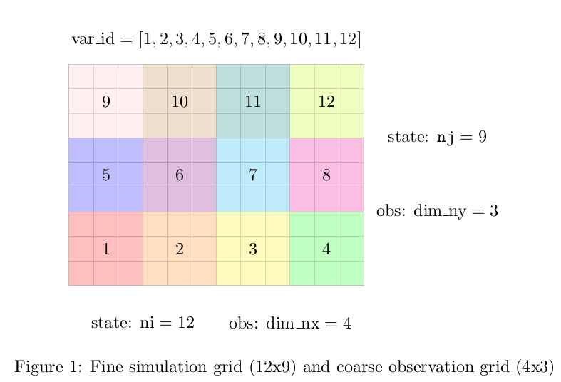
var_id#
var_id: (integer, dim=(dim_ny, dim_nx)) ID of cells with similar
observations.
Only used for multi-scale data
assimilation (turned on using
DA:point_obs).
The size of var_id is dim_obs.
var_id has equal values over model grid cells, which have range of
similar observations values from raw data over them.
The values of var_id have to start from var_id=1 for the first set
of observation values. Then, the consecutively higher integers should
be used (var_id=2,3,4,5 etc.) for other sets of observations. This
is important, as the maximal var_id will be used as “number of
var_id”.
If there are no observations over a set of grid cells, then a negative
var_id (integer) should assigned to this set.
dim_nx#
dim_nx: (integer) This is the x-dimension of the remote sensing
measurment in multi-scale Data Assimilation.
dim_ny#
dim_ny: (integer) This is the y-dimension of the remote sensing
measurment in multi-scale Data Assimilation.
Observation time flexibility#
Currently, in TSMP-PDAF there are a number input options that determine, when observations are read-in and assimilated:
Parflow:
TimeInfo.BaseUnitObservation file NetCDF variable
no_obs
The goal of this section is to show how these inputs can be used to create a flexible observation time input.
First, da_interval and TimeInfo.BaseUnit define the forward
integration step that is executed during on iteration of the main
TSMP-PDAF loop. This is the smallest time interval in your model and
it determines the counter, also for observation file names. So
da_interval should be small enough that each possible observation
can be attributed to one timestep.
Next, delt_obs is used to specify if data assimilation is not to be
called at every iteration/cycle of da_interval. If two available
observations are only da_interval apart, delt_obs has to be set to
1. However, suppose observations daily at noon, and da_interval is
one hour, then delt_obs could be chosen as 24.
Now, PDAF will be called every delt_obs iterations/cycles. However,
there is one last way of manipulating observation input, by setting
the NetCDF variable no_obs in the observation file to 0. In this
case, PDAF will skip the assimilation during that observation files
cycle. So, in principle, one could set delt_obs to 1, thus needing
an observation file at every cycle. At each timestep that is not
supposed to be assimilated, one could supply an alsmost-empty
observation file with just a single variable no_obs that has the
value 0. By this workaround, one obtains a fairly flexible
observation time input!
Example code for setting variable no_obs to zero in an existing NetCDF
file:
import scipy.io as scio

f = scio.netcdf_file("swc_obs.00001","a", mmap=False) # append
f.variables["no_obs"].assignValue(0)
f.close()
Example code for generating a minimal NetCDF observation file with
just one variable no_obs set to zero:
import numpy as np
import scipy.io as scio

f = scio.netcdf_file("swc_obs.00001","w", mmap=False) # write
f.createDimension("dim_noobs", 1)
f.createVariable("no_obs", np.int32, ["dim_noobs"])
f.variables["no_obs"].assignValue(0)
f.close()
da_interval#
da_interval: (float) Value for
da_interval used in the assimilation cycle
leading up to the observation file.
Specifying type of observation at compile time#
The following preprocessor variables let the user specify the expected observational input (i.e. ParFlow or CLM observations) at compile time (during the build-process). This may save some time during execution as certain parts of the source code are not accessed at all.
CLM observations: Set
ParFlow observations: Set